Although Pivot tables are very powerful, in the professional editions of excel there is one optional add-in more powerful and versatile than any other.
Practice File:
Transcript
It is called Power Pivot and in order to use it you have to first enable it.
Let’s do just that.
We click on the file Tab of the ribbon and then on options. There we select Add-ins. From the dropdown control we choose COM add-ins and we are presented with a list. If it is installed in our version of office, we should see the Microsoft Power Pivot for Excel on that list. We select it and click on OK.
A new tab appeared on our ribbon called Power Pivot. We click on it.
To be able to use Power Pivot we have to add some data to the data model.
Data model is a group of tables from a lot of different sources that can be combined by creating relationships.
So let’s add some data to our data model.
In the current sheet we have two different tables. We will add them both in the data model. We can add tables from different workbooks and different sources to our model. For simplicity reasons in this example we have both our data sources on the same sheet.
We select the first table and in the power pivot tab we click on “add to data model” button.
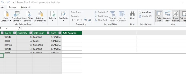
Our table has headers and Power Pivot opens showing it to us. Nothing impressive till now.
Let’s jump back to excel.
We add the second table to the data model
The second table appears in Power Pivot. We can see the previous table on the other tab.
We click on the button “Diagram view”. We see a diagram of our two tables.
Let’s create our first relationship.
Relationship between tables means that one field from one table is related with one field from another, thus the records with the same value on that field on each table are joined to each other.
The common fields, and so the most likely to relate, are the product fields. We drag the field from table1 to the field on table2. The relationship is created.
We can create a relationship without using the diagram view through a button of the design tab called “Create relationship”.
Let’s remove the relationship first. We right click on the line and select remove.
We now click on the create relationship button and select the product field on both tables.
We click ok and the relationship is there again.
The button manage relationships shows us a list of all our relationships and gives us the ability to edit or delete them.
But what is the practical use of all these.
We click on the home tab and then on pivot Table button. We have various choices. Let’s choose the first one.
The popup asks us where to place our pivot table. We choose the same sheet and after we click on ok we see the familiar environment of pivot tables.
With a small addition. The field list now consists of the fields in both our tables.
We select the price per item for columns and the product field for rows from table2. The sum of quantity, form table 1, is our values and the pivot table is ready.
As far as pivot tables are concerned this is not a so useful one. We used it for simplicity to show the steps needed in creating it.
The important thing here is that in our pivot table we depicted data from two different sources. By following the same steps, we can create a pivot table that gets data from numerous data sources related between them in various ways.
Power Pivot truly has no limits, other than our imagination and the amount of the data we feed it. We’ll dig in a little deeper on the next lesson and still we will have barely scratched the surface of its abilities.
