In this lesson we will try to explain and use a very useful feature of Pivot Tables. The creation of Calculated fields and items.
Practice File:
Transcript
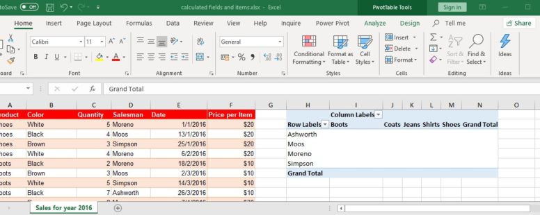
Let’s start by creating a pivot table. We select our data and click on pivot table. We add the product field on the columns and Salesman on the rows.
We want to show income, in dollars, that each salesman, produced, per product and in total.
This is where we have a small problem. To have the data we want on the pivot table we need to add a field in its values, which shows the income produced per sale. Unfortunately, we don’t have such a field.
We now face two options. We either create a new column in our original table to calculate the income per sale, and add it to our pivot table, or we create a calculated field.
You guessed right, we will choose the latter.
We click on our pivot table and from the analysis tab of the ribbon we click on the “field, items and sets” button. We choose Calculated field from the dropdown menu.
As name for the field we choose “income per sale”.
In the formula textbox we insert the field Quantity multiplied by the field “Price per Item” and then click on add.
A new field has just been added to our fields list. We drag it on the values area and we have the desired result.
We used a simple multiplication as formula for our field, but we can use any Excel function as complex as we want for the calculation of the field.
Having a closer look at our table we see that we have two products, (shoes and boots) which we would prefer to calculate together.
The options now are to change our original table and rename all boots and shoes records to “boots and shoes”, which we cannot do since their price is different.
To do the required calculation manually which could have some meaning in such a small dataset but none in every other case.
And to create a calculated Item, which it seems to be the only viable choice.
So a calculated item is a way to summarize two different sets of data items.
We click on the product headers of our pivot table and from the same dropdown menu as before we choose Calculated item.
We clicked on the product headers because, it is for the product field, we need a new item.
As name we type “Shoes and Boots” and as a formula we select the Shoes item added to the boots item.
In the formula field we can use any excel formula as long as the items we use are part of the product field.
We then click on add.
A new column just appeared with the name of the item we just created and the needed values depicted.
We can even use these items to filter our table and show just the income for the sale of shoes and boots.
There is a disadvantage though. If you noticed the totals column before and after the item insertion you would realize that the totals have changed since the shoes and boots data are calculated twice. This can be corrected by filtering out the Shoes and boots column when we want to have the real total values or by removing the new item altogether.
To do that we go to the same dropdown menu choice as before. We select the item we want to remove. And click on delete.
The totals have been corrected. We can do the same to remove the new field we created as well. Click on calculated field and then choose the new field, and click on delete.
Analyzing data can be fun, right?