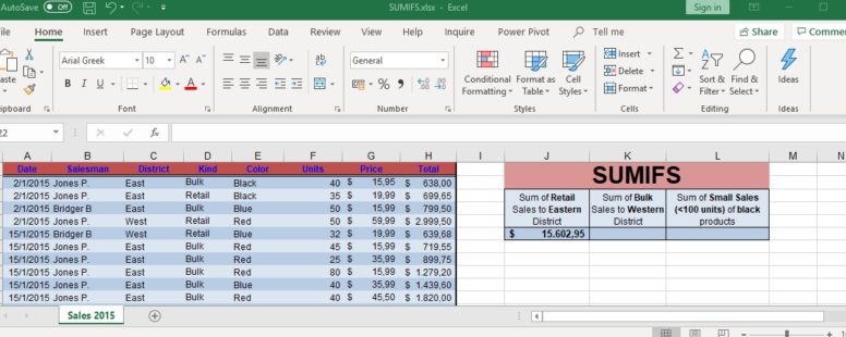
The SUMIFS function adds the cells that meet all its multiple criteria. Even though its logical elements, it is part of the Mathematical functions of Excel.
We have prepared a tutorial on the SUMIFSfunction to explain it in a bit more detail.
The syntax of the function is the following:
SUMIFS(Sum_range, Criteria_range1, Criteria1, [Criteria_range2, Criteria2, ...])
Sum_range: The cell range we want to sum.
Criteria_range1, Criteria_range2, … : Criteria_range1 is required. The rest (up to 127) are optional. They are the range of cells that have to meet certain criteria.
Criteria1, Criteria2, … : Same as above only the first is required. The rest (up to 127) are optional. You cannot enter Criteria without a Criteria_range and vice versa. They contain the criterion (expression, number, reference…) that the respective criterion_range has to meet.
If a cell in a criteria range is empty, SUMIFS considers it a zero.
TRUE is considered 1 and FALSE 0.
Each Criteria_range must be the same size and shape as Sum_range.
You can use the wildcard characters, question mark (?) and asterisk (*), in criteria. If you want to find an actual question mark or asterisk, type a tilde (~) before the character.
Click on the button to practice using this function, with the help of our Online Assessment Tool:
Here are two examples of how to use the SUMIFS function:
In the cell H4 calculate the sum of all orders with amount greater than 40, which were placed after 2/1/2004.
Use the proper formula in the cell I2, to calculate the sum of the Total of Sales, from the eastern district, with less than 55 units sold.
