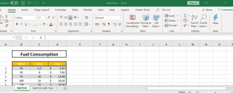
The MATCH function searches for a specified item in a range of cells, and then returns the relative position of that item in the range .
We have prepared a tutorial on the MATCH function to explain it in a bit more detail.
The syntax of the function is the following:
MATCH(lookup_value, lookup_array, [match_type])
lookup_value : The value that you want to match in lookup_array.
lookup_array : The range of cells being searched.
match_type: Optional. The number -1, 0, or 1.
- The default value is 1. It finds the largest value that is less than or equal to lookup_value.
- The value 0 finds the first value that is exactly equal to lookup_value.
- The value -1 finds the smallest value that is greater than or equal to lookup_value.
MATCH return the position of the matched value and not the value itself
MATCH is case insensitive when matching text values
If no match is found an error #N/A is returned.
You can use the wildcard characters, question mark (?) and asterisk (*), in criteria. If you want to find an actual question mark or asterisk, type a tilde (~) before the character.
Click on the button to practice using this function, with the help of our Online Assessment Tool:
Here is an example of how to use the MATCH function:
Use the proper formula to match the position of the table where the products of the cells E7:E8 are found, and show the respected values in the cells F7:F8.
