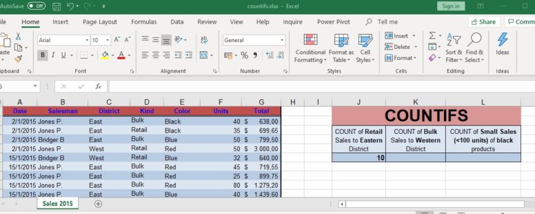
The COUNTIFS function counts the number of times certain criterias are met. Even though its logical elements, it is part of the Statistical functions of Excel.
We have prepared a tutorial on the COUNTIFS function to explain it in a bit more detail.
The syntax of the function is the following:
COUNTIFS(Criteria_range1, Criteria1, [Criteria_range2, Criteria2, ...])
Criteria_range1, Criteria_range2, … : Criteria_range1 is required. The rest (up to 127) are optional. They are the range of cells that have to meet certain criteria.
Criteria1, Criteria2, … : Same as above only Criteria1 is required. The rest (up to 127) are optional. You cannot enter Criteria without a Criteria_range and vice versa. They contain the criterion (expression, number, reference…) that the respective criterion_range has to meet.
If a cell in a criteria range is empty, COUNTIFS considers it a zero.
Each Criteria_range must be the same size and shape as Criteria_range1 .
You can use the wildcard characters, question mark (?) and asterisk (*), in criteria. If you want to find an actual question mark or asterisk, type a tilde (~) before the character.
Click on the button to practice using this function, with the help of our Online Assessment Tool:
Here are examples of how to use the COUNTIFS function:
In the cell H4 calculate the count of the orders, with amount greater than 40 that were placed after February 1st 2004.
Use the proper formula in the cell I2, to calculate the count of the Total of Sales, from the eastern district, with less than 80 units sold.
