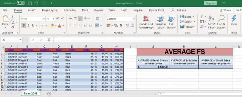
The AVERAGEIFS function returns the arithmetic mean (average) of all the cells that meet all its multiple criteria. Even though its logical elements, it is part of the Statistical functions of Excel.
We have prepared a tutorial on the AVERAGEIFS function to explain it in a bit more detail.
The syntax of the function is the following:
AVERAGEIFS(Average_range, Criteria_range1, Criteria1, [Criteria_range2, Criteria2, ...])
Average_range: The cell range for which we want to calculate the arithmetic mean.
Criteria_range1, Criteria_range2, … : Criteria_range1 is required. The rest (up to 127) are optional. They are the range of cells that have to meet certain criteria.
Criteria1, Criteria2, … : Same as above only the first is required. The rest (up to 127) are optional. You cannot enter Criteria without a Criteria_range and vice versa. They contain the criterion (expression, number, reference…) that the respective criterion_range has to meet.
If Average_range is blank or text, AVERAGEIFS returns the #DIV0! error.
If a cell in a criteria range is empty, AVERAGEIFS considers it a zero.
TRUE is considered 1 and FALSE 0.
Each Criteria_range must be the same size and shape as Average_range.
If cells in Average_range are not numbers, AVERAGEIFS returns the #DIV0! error.
If there aren’t any cells that meet all the criteria, AVERAGEIFS returns the #DIV/0! error.
You can use the wildcard characters, question mark (?) and asterisk (*), in criteria. If you want to find an actual question mark or asterisk, type a tilde (~) before the character.
The AVERAGEIFS function is used to measure Central Tendency.
Click on the button to practice using this function, with the help of our Online Assessment Tool:
Here is an example of how to use the AVERAGEIFS function:
Use the proper formula in the cell I2, to calculate the average of the Total of Sales, from the western district, with greater than 100 units sold.
