The INDEX function is one of the most interesting functions in excel. It can be combined with many other functions to help you out of some difficult situations.
Practice File:
Transcript
Let’s start with the basics.
It comes in two formats. An array format and a range format.
The array format looks up a reference to a cell within a single, cell range.
Suppose we want, in our example, to calculate in cell c9 the grade of student 2 (Mary) to lesson 3 (chemistry).
We type the name of the function and open the parenthesis. Notice the two different formats of the function.
We select the cell range that shows the grades and then the row (number 2) and the column (number 3).
As expected we have the grade of Mary in Chemistry which is 6.
If one of the row or column numbers are set to zero, then INDEX returns the whole column or row respectively.
Suppose that we want to calculate the average grade of Mary using INDEX. We alter our formula by setting the column number to 0, thus making INDEX to return to us the whole second row of data. We enclose this in an Average function and there we are. The average grade of Mary.
We should note here that we can’t set both row and column number to zero, because it would result in an error.
It looks rather easy till now, and not that interesting.
Let’s see now the range format of the function.
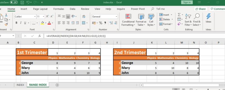
In our next sheet we can see the grades of the students for all trimesters.
Using the range format, we can add to our INDEX function the cell ranges with the grades for each trimester.
We will calculate the average grade of Mary for the first trimester in cell C17.
We type the average function and inside it, we will enclose an index function. For the first attribute of the index function we have to provide the range. Our range originates from three different cell ranges. So we open a parenthesis and provide the three different cell areas divided by commas, and then close the parenthesis.
Then we type the row number which is 2 for Mary. The column number is 0 since we want the whole row, and then as we can see from the auto complete we are required to enter an area number. The area number refers to the cell areas we entered before and is relative to the order we entered them. So for the first trimester we enter 1. The area number is optional and if skipped it defaults to 1.
We close the parenthesis and we have the desired result as on the previous sheet.
If we want to see the average of another trimester we just change the area number to its respective one. So for the second trimester we enter 2 and for the third trimester we enter 3.
I told you at the beginning that index is one of the most interesting functions in excel, and I’m sure that you might feel a bit disappointed.
Bear with me for a few more lessons and you will find out that index combined with match make up the best lookup formulas there are and probably the ones you are going to use every time. I know I do.
