In Excel the manipulation and management of data is not limited to complex calculations.
It is certain that at some point everybody needs to alter the form and layout of their data, in order for them to be more readable, or answer to some specific visual requirements.
The ability to transpose our data is such a need.
Practice File:
Transcript
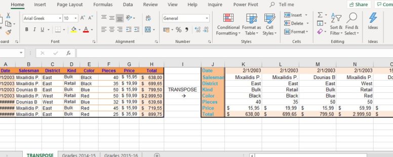
In our example we can see two tables. These tables are filled with the exactly the same data. Their only difference is that the rightmost table was produced by the vertical arrangement of the leftmost one.
There are two ways to achieve this.
Let’s go to the next worksheet which shows the monthly grades of a student for the school year 2014 – 2015.
The data consists of a 12 columns to 7 rows table. Suppose we need the months to be row headers and the courses to be column headers.
So we need the table to be 7 columns wide and 12 rows tall. We select a cell area that fits these criteria. In our example we will use the area from N1 to T12.
We then type the equals sign and the TRANSPOSE function. We type the source array enclosed in parenthesis but do not press ENTER.
Transpose can only be used in array formulas. Array formulas is a subject for another lesson, but their common characteristic is that to finish an array formula you don’t press Enter but CTRL+SHIFT+ENTER.
By pressing this key combination, we see this result. The arrangement of the table has changed.
If we alter a grade at the leftmost table, for example the physics grade for September to 7, we observe that the same change happens to the rightmost table.
These two tables are linked which is the main advantage of the transpose function.
But with a closer look at our new table we can see that it did not inherit the formatting and the style of its parent table.
This means we will have to stylize the new table from scratch which in some cases could prove to be a really time consuming job especially if we had formatting rules and conditions already applied to the parent table.
we will choose a different approach.
We select the table and copy it to the clipboard.
Then we select the cell N1 and use the transpose paste option.
We can see that all formatting has been preserved.
But if we change the grade of Physics for September in the leftmost table, we will notice that the respective cell in the rightmost table remains unchanged. We have to change the grade manually.
We will see though that the formatting rule was preserved and the cell background is no longer red.
So as we can see this method makes a copy of the parent array arranged vertically and the two tables are not linked in any way.
