Pivot charts in Excel are the visual representation of pivot tables. They are connected to each other and every change on the table affects the chart and vice versa.
Practice File:
Transcript
They have all the basic functionality of a standard excel chart plus some extra features.
There are two ways to create a Pivot chart. The first is to create a Pivot Table and then Insert a Pivot chart based on that table, and the other is to insert them together. To access both ways we have to click on the insert tab of the ribbon and from the pivot Chart dropdown menu select one or the other.
We select to insert both to save us some time.
We either choose a cell to insert them or insert them into a new sheet.
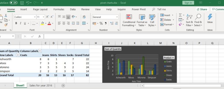
Then we set the Product field as column, the Salesman as Row and the Sum of quantity as values.
If we have the chart selected instead of columns and rows we drag the fields to the Legend and Category areas respectively.
The visual differences from a regular chart are these 3 grayed fields on the chart. We can use the Product and Salesman fields to filter the results of the pivot table and the chart, and the sum of Quantity field to change its properties.
For example, let’s change the value field to depict the count of sales instead of the sum. We right click on the field and select properties and then count.
Both the chart and the table have changed to reflect our new setting.
Let’s filter the chart now to not show Mr. Simpson and the sales for shirts.
Again the chart and the table change together. The same filters can be applied to the table and be depicted on the chart instantly. Let’s return our chart to its original state using the pivot table filters and options.
First remove the filters. And then change back to showing the sum instead of the count of quantities.
Every functionality that exists on a regular chart is present here as well. We can change the type of the chart, the style, the colors and pretty much anything we like on the design of the chart.